Spin Orbit Coupling

Creation of 2D SOC

First realization

They realize 2D SOC in Rubidium atoms . The engineered Hamiltonian: $\hat H = \left[ \frac{\hbar k^2}{2m} +V_{latt}(x,z)\right]I+M_x(x,z)\sigma_x+M_y(x,z)\sigma_y+m_z\sigma_z$, where Mx and My are periodic Raman coupling potentials, mz is a tunable Zeeman constant. The lattice potential is spin-independent, the hopping between nearest sights conserves the spin. Mx and My induce hopping that flips the spin.

Square lattice

The experimental realization is published here . 2 orthogonal beams are sent back and forth to create a square lattice: $V_{latt}=V_0\cos^2(k_0 x)+V_0\sin^2(k_0 y)$. The total Hamiltonian of the system reads as 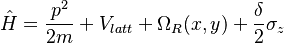$\hat H = \frac{p^2}{2m}+V_{latt}+\Omega_{R}(x,y)+\frac{\delta}{2}\sigma_z$, where δ is the two-photon detuning. This Hamiltonian exhibits precise inversion and C4 symmetries. By tuning the phase between two beams δφ it is possible to transition from 1D to 2D SOC. For phases δφ=0, π, they demonsrate 1D SOC. For phases δφ=±π/2 they have symmetrical 2D SOC.

1. They measure the lifetime of the BEC in 2D SOC, they find it to be 1-3s depending on the lattice depth.
2. They measure the stripe and magnetic phases. They build the hystograms for different magnetizations, for the one they have a single peak at M=0 they call it a stripe phase. For the magnetic phase they have two sharp peaks at M=±1. The phase transition point is found as $\sqrt{\langle M_0 \rangle}$ as a function of Ω, where they find a turning point.
3. They measure band topology.

.