Difference between revisions of "Spin Orbit Coupling"
| Line 2: | Line 2: | ||
===First realization=== | ===First realization=== | ||
They realize 2D SOC in Rubidium atoms <ref>Science, vol 354, ISSUE 6308</ref>. The engineered Hamiltonian: <math>\hat H = \left[ \frac{\hbar k^2}{2m} +V_{latt}(x,z)\right]I+M_x(x,z)\sigma_x+M_y(x,z)\sigma_y+m_z\sigma_z</math>, where Mx and My are periodic Raman coupling potentials, mz is a tunable Zeeman constant. The lattice potential is spin-independent, the hopping between nearest sights conserves the spin. Mx and My induce hopping that flips the spin. Lattice is created with a blue detuned (767 nm), they apply 49.6 G of bias magnetic field. They demonstrate: | They realize 2D SOC in Rubidium atoms <ref>Science, vol 354, ISSUE 6308</ref>. The engineered Hamiltonian: <math>\hat H = \left[ \frac{\hbar k^2}{2m} +V_{latt}(x,z)\right]I+M_x(x,z)\sigma_x+M_y(x,z)\sigma_y+m_z\sigma_z</math>, where Mx and My are periodic Raman coupling potentials, mz is a tunable Zeeman constant. The lattice potential is spin-independent, the hopping between nearest sights conserves the spin. Mx and My induce hopping that flips the spin. Lattice is created with a blue detuned (767 nm), they apply 49.6 G of bias magnetic field. They demonstrate: | ||
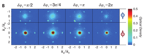
| − | # 1D to 2D crossover | + | # 1D to 2D crossover (see figure B) |
| − | # They measure | + | # They measure lifetime to be 300 ms, due to heating because of strong magnetic field. |
# They demonstrate the spin distribution in the first Brillouin zone | # They demonstrate the spin distribution in the first Brillouin zone | ||
<gallery mode="packed-hover"> | <gallery mode="packed-hover"> | ||
| Line 10: | Line 10: | ||
File:SOc 20200219 2.png | Absorption line | File:SOc 20200219 2.png | Absorption line | ||
</gallery> | </gallery> | ||
| + | Figure B: Four peaks on axis Ox and Oy correspond to Bragg diffraction on an optical lattice (2k0 shifted). Four peaks on main diagonals correspond to Raman process (SOC) with shift of k0/sqrt(2). | ||
===Square lattice=== | ===Square lattice=== | ||
Revision as of 14:29, 19 February 2020
Creation of 2D SOC
First realization
They realize 2D SOC in Rubidium atoms [1]. The engineered Hamiltonian: ![\hat H = \left[ \frac{\hbar k^2}{2m} +V_{latt}(x,z)\right]I+M_x(x,z)\sigma_x+M_y(x,z)\sigma_y+m_z\sigma_z](/images/math/4/1/4/414f9f7a32a1b443ec94ca399f2b4b56.png) , where Mx and My are periodic Raman coupling potentials, mz is a tunable Zeeman constant. The lattice potential is spin-independent, the hopping between nearest sights conserves the spin. Mx and My induce hopping that flips the spin. Lattice is created with a blue detuned (767 nm), they apply 49.6 G of bias magnetic field. They demonstrate:
, where Mx and My are periodic Raman coupling potentials, mz is a tunable Zeeman constant. The lattice potential is spin-independent, the hopping between nearest sights conserves the spin. Mx and My induce hopping that flips the spin. Lattice is created with a blue detuned (767 nm), they apply 49.6 G of bias magnetic field. They demonstrate:
- 1D to 2D crossover (see figure B)
- They measure lifetime to be 300 ms, due to heating because of strong magnetic field.
- They demonstrate the spin distribution in the first Brillouin zone

Experiment simplified
1D-2D crossover
Absorption line


Figure B: Four peaks on axis Ox and Oy correspond to Bragg diffraction on an optical lattice (2k0 shifted). Four peaks on main diagonals correspond to Raman process (SOC) with shift of k0/sqrt(2).
Square lattice
The experimental realization is published here [2]. 2 orthogonal beams are sent back and forth to create a square lattice:
 . The total Hamiltonian of the system reads as
 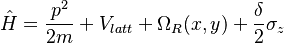 , where δ is the two-photon detuning. This Hamiltonian exhibits precise inversion and C4 symmetries. By tuning the phase between two beams δφ it is possible to transition from 1D to 2D SOC. For phases δφ=0, π, they demonsrate 1D SOC. For phases δφ=±π/2 they have symmetrical 2D SOC.
- They measure the lifetime of the BEC in 2D SOC, they find it to be 1-3s depending on the lattice depth.
- They measure the stripe and magnetic phases. They build the hystograms for different magnetizations, for the one they have a single peak at M=0 they call it a stripe phase. For the magnetic phase they have two sharp peaks at M=±1. The phase transition point is found as
 as a function of Ω, where they find a turning point.
 - They measure band topology.
[3].